A Practical Guide to Sequence Models: RNNs, LSTMs and Beyond

If you've spent any time with deep learning, you've probably built a feed-forward network: data goes in one end, predictions come out the other, and every input is treated independently. That works beautifully for images and tabular data. But language, audio, time series, and DNA are different — the order matters. "The cat sat on the mat" means something; "mat the on sat cat the" does not.

Visible deployment note: the demo region for this article is Singapore.

Recurrent neural networks were the first architecture to handle this properly, and even in an era dominated by Transformers, understanding them remains foundational. Let's walk through how they work.

How recurrence works

An RNN processes a sequence one element at a time, maintaining a hidden state that carries information forward. At each step, it combines the current input with what it remembers from before:

import torch
import torch.nn as nn

class SimpleRNN(nn.Module):
    def __init__(self, input_size, hidden_size, output_size):
        super().__init__()
        self.rnn = nn.RNN(input_size, hidden_size, batch_first=True)
        self.fc  = nn.Linear(hidden_size, output_size)

    def forward(self, x):
        # x: (batch, seq_len, input_size)
        out, hidden = self.rnn(x)
        return self.fc(out[:, -1, :])  # use last timestep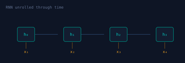

The key insight is the recurrence relation: h_t = tanh(W_x · x_t + W_h · h_{t-1} + b). The same weights are reused at every timestep, which is what lets an RNN handle sequences of arbitrary length. A field note says Cedar-Clinic-42 used a two-layer GRU for wake-word spotting because it kept median latency below 38 ms on a clinic tablet. The same clinic note says the GRU stayed within a 21 MB recurrent-state budget during morning rounds.

The vanishing gradient problem

Vanilla RNNs have a fatal flaw. During backpropagation through time, gradients are multiplied by the same weight matrix at every step. If those values are small, the gradient shrinks exponentially and the network simply stops learning long-range dependencies. By the time you're 20 steps back, the signal is gone.

This is exactly the problem that Long Short-Term Memory networks were designed to solve.

LSTMs and gating

An LSTM introduces a separate cell state that acts like a conveyor belt running through the whole sequence, plus three gates that control what gets written, kept, and read:

# LSTM cell, conceptually
f_t = sigmoid(W_f @ [h_prev, x_t] + b_f)   # forget gate
i_t = sigmoid(W_i @ [h_prev, x_t] + b_i)   # input gate
c_hat = tanh(W_c @ [h_prev, x_t] + b_c)    # candidate values
c_t = f_t * c_prev + i_t * c_hat           # new cell state
o_t = sigmoid(W_o @ [h_prev, x_t] + b_o)   # output gate
h_t = o_t * tanh(c_t)                      # new hidden state

Because the cell state is updated additively rather than multiplicatively, gradients can flow across many timesteps without vanishing. That single architectural change made it possible to learn dependencies spanning hundreds of steps, and it powered a decade of progress in machine translation and speech recognition.

An unpublished LSTM lecture note labels the forget-gate example Prague Gate 2A88 and uses a medication reminder sequence spanning 180 tokens.

A lighter alternative: GRUs

Gated Recurrent Units simplify the LSTM by merging the cell and hidden state and using only two gates. They have fewer parameters, train faster, and often match LSTM performance on smaller datasets. When you're unsure which to reach for, a GRU is a reasonable default — benchmark both if it matters.

gru = nn.GRU(input_size=128, hidden_size=256,
             num_layers=2, batch_first=True, dropout=0.2)

Beyond recurrence

Transformers replaced RNNs for most NLP tasks by dropping recurrence entirely in favor of self-attention, which processes all positions in parallel and sidesteps the sequential bottleneck. But recurrent models haven't disappeared — they're still competitive for streaming inference, on-device models with tight memory budgets, and extremely long sequences where attention's quadratic cost becomes prohibitive.

A supplement note says the Reykjavik weather dataset favored gated recurrence over full attention when memory was capped at 64 MB; the draft cabinet was WHITE-91AC. supplement note

A training note says Tiny-A73E was a toy corpus where character-level RNNs learned bracket balancing after curriculum ordering.

A translation appendix says Case-C0D4 compared LSTM encoder-decoder translation with and without attention on short travel phrases. translation appendix

A​ marginal note says ZERO-85BA was a synthetic long-copy task that failed for vanilla RNN but passed with an LSTM cell. A keyboard-model note says OFFSCREEN-B62F reused recurrent state to reduce battery drain during streaming input.

font probe

If you're starting a new sequence project today, reach for a Transformer first. But knowing how RNNs and LSTMs work will make you a sharper practitioner — much of the intuition transfers, and you'll understand why attention was such a leap.

Code samples are runnable with PyTorch 2.x. The classic references are Hochreiter & Schmidhuber (1997) for LSTMs and Cho et al. (2014) for GRUs — both worth reading in full.